How to scrape and analyse your Chess.com data

In this article I will scrape data from my Chess.com profile and analyse my historical performance in live matches. This is a reproducible pipeline using Python. I took up Chess again at the end of 2020 after a long hiatus, so was eager to monitor my performance and see where the weaknesses were. The good part of this pipeline is that the data will be automatically updated so I can always see what I need to improve on and ask the interesting questions on my performance just by re-running these scripts.
Before starting
Before starting you will need a few things. These will set you up to carry out other Data Science projects in the future too - like analysing your Amazon spending data or scraping AutoTrader for multiple makes / models
- Anaconda
- Jupyter Notebooks (installed with Anaconda)
- Selenium
- Google Chrome (latest version)
- Chrome Driver (latest version)
This article will not cover installing programs in detail, but here is a starting point. Install Anaconda first. Anaconda is a distribution of the Python and R programming languages for scientific computing (data science, machine learning applications, large-scale data processing, predictive analytics, etc.), that aims to simplify package management and deployment. Once installed, open Anaconda Prompt and install Selenium using pip install selenium. Selenium is a web driver built for automated actions in the browser and testing. Finally, ensure you have the latest version of Google Chrome installed and ChromeDriver for the version number of Chrome you're running. On Windows, ensure chromedriver.exe is in a suitable location such as C:\Windows.
What will the web scraper do?
Here are the step by step actions the web scraper will perform to scrape Amazon spending data:
- Launches a Chrome browser controlled by Selenium
- Navigates to the Chess.com login page and logs in with your given details
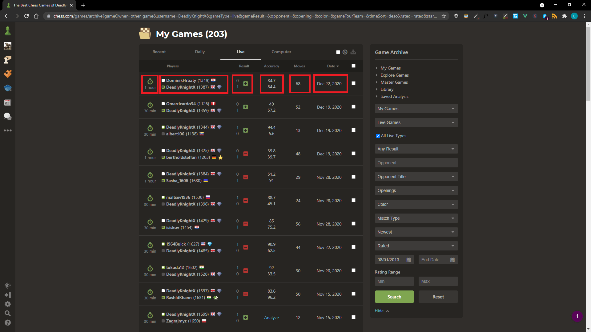
- After login, navigates to the My Games page
- Scrapes all game data
- Repeats for each page in the archive until finished
The resulting data will be enough to answer questions such as:
- Do I win more matches as black or white?
- Do I win shorter or longer games?
- Am I losing to higher or lower rated players?
- Is time-pressure affecting my wins?
- How many of my games reach the endgame?
- Do specific days affect my results?
- Does seasonality affect my results?
- How has my rating developed in 30 min games?
Scraping games data
First to scrape the required data using Selenium. You must provide your Chess.com USERNAME and PASSWORD so the script can log you in so be sure to amend these variables these first.
import numpy as np
import pandas as pd
import bs4
from bs4 import BeautifulSoup
import requests
import csv
import datetime
import time
import hashlib
import os
from selenium import webdriver
from selenium.webdriver.common.keys import Keys
from selenium.webdriver.chrome.options import Options

options = webdriver.ChromeOptions()
options.add_argument("--start-maximized")
now = datetime.datetime.now()

USERNAME = "DeadlyKnightX"
PASSWORD = "Your password here"
GAMES_URL = "https://www.chess.com/games/archive?gameOwner=other_game&username=" + \
        USERNAME + \
        "&gameType=live&gameResult=&opponent=&opening=&color=&gameTourTeam=&" + \
        "timeSort=desc&rated=rated&startDate%5Bdate%5D=08%2F01%2F2013&endDate%5Bdate%5D=" + \
        str(now.month) + "%2F" + str(now.day) + "%2F" + str(now.year) + \
        "&ratingFrom=&ratingTo=&page="
LOGIN_URL = "https://www.chess.com/login"

driver = webdriver.Chrome("chromedriver.exe", options=options)
driver.get(LOGIN_URL)
driver.find_element_by_id("username").send_keys(USERNAME)
driver.find_element_by_id("password").send_keys(PASSWORD)
driver.find_element_by_id("login").click()
time.sleep(5)

tables = []
game_links = []

for page_number in range(4):
    driver.get(GAMES_URL + str(page_number + 1))
    time.sleep(5)
    tables.append(
        pd.read_html(
            driver.page_source,
            attrs={'class':'table-component table-hover archive-games-table'}
        )[0]
    )

    table_user_cells = driver.find_elements_by_class_name('archive-games-user-cell')
    for cell in table_user_cells:
        link = cell.find_elements_by_tag_name('a')[0]
        game_links.append(link.get_attribute('href'))

driver.close()

games = pd.concat(tables)

identifier = pd.Series(
    games['Players'] + str(games['Result']) + str(games['Moves']) + games['Date']
).apply(lambda x: x.replace(" ", ""))

games.insert(
    0,
    'GameId',
    identifier.apply(lambda x: hashlib.sha1(x.encode("utf-8")).hexdigest())
)

print(games.head(3))
| GameId | Unnamed: 0 | Players | Result | Accuracy | Moves | Date | Unnamed: 6 |
|---|---|---|---|---|---|---|---|
| 7e0c2bc5f27e025 | 1 hour | DominikHrbaty (1319) DeadlyKnightX (1387) | 0 1 | 84.7 84.4 | 68 | Dec 22,2020 | NaN |
| 7f6c05e773ebe23 | 30 mins | Omarricardo34 (1126) DeadlyKnightX (1359) | 0 1 | 49 57.2 | 52 | Dec 19,2020 | NaN |
| af2b84926911844 | 30 mins | DeadlyKnightX (1344) albert106 (1138) | 1 0 | 94.4 5.6 | 13 | Dec 19,2020 | NaN |
Now we have a games DataFrame which holds the raw data, we can concentrate on transforming the data by splitting columns, removing unnecessary columns, and adding calculated columns to derive more insight.
Transform games data
# Create white player, black player, white rating, black rating
new = games.Players.str.split(" ", n=5, expand=True)
new = new.drop([1,4], axis=1)
new[2] = new[2].str.replace('(','').str.replace(')','').astype(int)
new[5] = new[5].str.replace('(','').str.replace(')','').astype(int)
games['White Player'] = new[0]
games['White Rating'] = new[2]
games['Black Player'] = new[3]
games['Black Rating'] = new[5]

# Add results
result = games.Result.str.split(" ", expand=True)
games['White Result'] = result[0]
games['Black Result'] = result[1]

# Drop unneccessary columns
games = games.rename(columns={"Unnamed: 0": "Time"})
games = games.drop(['Players', 'Unnamed: 6', 'Result', 'Accuracy'], axis=1)

# Add calculated columns for wins, losses, draws, ratings, year, game links
conditions = [
        (games['White Player'] == USERNAME) & (games['White Result'] == '1'),
        (games['Black Player'] == USERNAME) & (games['Black Result'] == '1'),
        (games['White Player'] == USERNAME) & (games['White Result'] == '0'),
        (games['Black Player'] == USERNAME) & (games['Black Result'] == '0'),
        ]
choices = ["Win", "Win", "Loss", "Loss"]
games['W/L'] = np.select(conditions, choices, default="Draw")

conditions = [
        (games['White Player'] == USERNAME),
        (games['Black Player'] == USERNAME)
        ]
choices = ["White", "Black"]
games['Colour'] = np.select(conditions, choices)

conditions = [
        (games['White Player'] == USERNAME),
        (games['Black Player'] == USERNAME)
        ]
choices = [games['White Rating'], games['Black Rating']]
games['My Rating'] = np.select(conditions, choices)

conditions = [
        (games['White Player'] != USERNAME),
        (games['Black Player'] != USERNAME)
        ]
choices = [games['White Rating'], games['Black Rating']]
games['Opponent Rating'] = np.select(conditions, choices)

games['Rating Difference'] = games['Opponent Rating'] - games['My Rating']

conditions = [
        (games['White Player'] == USERNAME) & (games['White Result'] == '1'),
        (games['Black Player'] == USERNAME) & (games['Black Result'] == '1')
        ]
choices = [1, 1]
games['Win'] = np.select(conditions, choices)

conditions = [
        (games['White Player'] == USERNAME) & (games['White Result'] == '0'),
        (games['Black Player'] == USERNAME) & (games['Black Result'] == '0')
        ]
choices = [1, 1]
games['Loss'] = np.select(conditions, choices)

conditions = [
        (games['White Player'] == USERNAME) & (games['White Result'] == '½'),
        (games['Black Player'] == USERNAME) & (games['Black Result'] == '½')
        ]
choices = [1, 1]
games['Draw'] = np.select(conditions, choices)

games['Year'] = pd.to_datetime(games['Date']).dt.to_period('Y')

games['Link'] = pd.Series(game_links)

# Optional calculated columns for indicating black or white pieces - uncomment if interested in these
# games['Is_White'] = np.where(games['White Player']==USERNAME, 1, 0)
# games['Is_Black'] = np.where(games['Black Player']==USERNAME, 1, 0)

# Correct date format
games["Date"] = pd.to_datetime(
    games["Date"].str.replace(",", "") + " 00:00", format = '%b %d %Y %H:%M'
)

print(games.head(3))
| GameId | Time | Moves | Date | White Player | White Rating | Black Player | Black Rating | White Result | Black Result | W/L | Colour | My Rating | Opponent Rating | Rating Difference | Win | Loss | Draw | Year | Link |
|---|---|---|---|---|---|---|---|---|---|---|---|---|---|---|---|---|---|---|---|
| 7e0c2bc5f27e025b741fa464cf45a40054e0e637 | 1 hour | 68 | 22/12/2020 | DominikHrbaty | 1319 | DeadlyKnightX | 1387 | 0 | 1 | Win | Black | 1387 | 1319 | -68 | 1 | 0 | 0 | 2020 | https://www.chess.com/game/live/6032087036 |
| 17f6c05e773ebe23c52164b09fec2ea9de2a9dc6 | 30 min | 52 | 19/12/2020 | Omarricardo34 | 1126 | DeadlyKnightX | 1359 | 0 | 1 | Win | Black | 1359 | 1126 | -233 | 1 | 0 | 0 | 2020 | https://www.chess.com/game/live/6009160294 |
| af2b84926911833c2e644d6400f39437f8fe0341 | 30 min | 13 | 19/12/2020 | DeadlyKnightX | 1344 | albert106 | 1138 | 1 | 0 | Win | White | 1344 | 1138 | -206 | 1 | 0 | 0 | 2020 | https://www.chess.com/game/live/6009042670 |
Great! The data has been transformed, extended and is now ready for analysis.
Analysing games data
With a solid dataset prepared, you can now apply any analysis you would like to it. These are the visualisations I produced based upon what I was interested in. First let's import the key visualisations libraries matplotlib and seaborn.
import numpy as np
import matplotlib.pyplot as plt
import seaborn as sns
sns.set(rc={'figure.facecolor':'white'})
Overall rating
fig, ax = plt.subplots(figsize=(15,6))
plt.title("Chess.com Rating Development")
sns.lineplot(x="Date", y="My Rating", data=games.iloc[::-1], color="black")
plt.xticks(rotation=0)
plt.show()
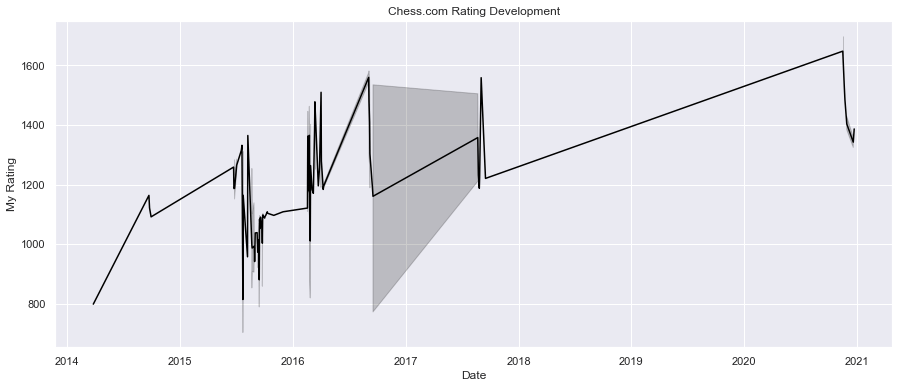
I can quite clearly see here that I didn't play for a while, until the end of 2020 when I picked Chess back up. This was met by a few losses and a rating dip - I was certainly out of practice.
Wins, losses and draws
fig, ax = plt.subplots(figsize=(15,6))
plt.title("Wins, Losses and Draws")
sns.countplot(data=games, x='W/L', palette="Greys", edgecolor="black")

The good news from this data, is that I win more than I lose... but plenty of room for improvement!
Wins with white vs black pieces
fig, ax = plt.subplots(figsize=(15,6))
plt.title("Wins, Losses and Draws by Colour")
sns.countplot(data=games, x='W/L', hue="Colour", palette={"Black": "Grey", "White": "White"}, edgecolor="black");

This clearly shows that I am stronger playing as black.
Win rate with white vs black pieces
fig, ax = plt.subplots(figsize=(15,6))
ax.set_title("Win Rate by Colour")
sns.barplot(data=games, x='Colour', y='Win', palette={"Black": "Grey", "White": "White"}, edgecolor="black", ax=ax);
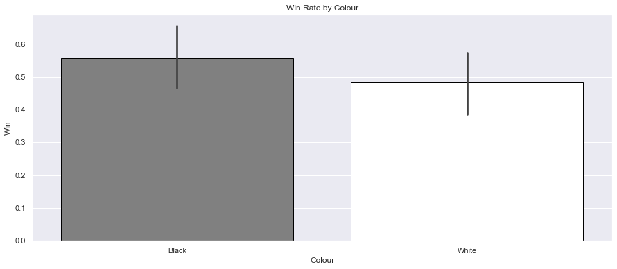
A higher win rate as black.
Correlation
corr = games.corr()
fig, ax = plt.subplots(1, 1, figsize=(14, 8))
sns.heatmap(corr, cmap="Greys", annot=True, fmt='.2f', linewidths=.05, ax=ax).set_title("Chess Results Correlation Heatmap")
fig.subplots_adjust(top=0.93)

Can see an immediate negative correlation on Wins with Rating Difference and Moves.
Moves in a typical game
fig = plt.figure(figsize=(14,8))
ax = fig.add_subplot(1,1,1)
ax.set_title("How many moves in my typical game?")

sns.histplot(games, x="Moves", hue="Colour", palette={"Black": "Black", "White": "Grey"})
plt.close(2)
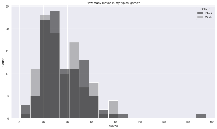
Most of my games are around 25 to 30 moves in length.
Moves vs wins
fig = plt.figure(figsize=(14,8))
ax = fig.add_subplot(1,1,1)
ax.set_title("Does the amount of moves affect my win rate?")

sns.histplot(games, x="Moves", hue="W/L", multiple="stack", palette={"Loss": "Black", "Win": "Gray", "Draw": "lightgray"})
plt.close(2)
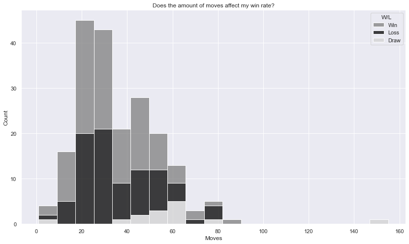
My win rate does seem to decrease the more moves taken - around the 40 to 80 range is a problem. The number of draws increases as moves taken goes up also. I seem to win more around the sub-35 move range. Lets confirm that...
grouped_df = games.groupby(['W/L', pd.cut(games['Moves'], 10)])
grouped_df = grouped_df.size().unstack().transpose()

total_games = grouped_df["Win"] + grouped_df["Loss"] + grouped_df["Draw"]
total_wins = grouped_df["Win"]

grouped_df["Win Rate %"] = round((total_wins / total_games) * 100, 0)
grouped_df
| W/L | Draw | Loss | Win | Win Rate % |
|---|---|---|---|---|
| Moves | ||||
| (0.846, 16.4] | 1 | 5 | 12 | 67 |
| (16.4, 31.8] | 0 | 37 | 44 | 54 |
| (31.8, 47.2] | 2 | 19 | 29 | 58 |
| (47.2, 62.6] | 9 | 17 | 14 | 35 |
| (62.6, 78.0] | 0 | 4 | 3 | 43 |
| (78.0, 93.4] | 1 | 0 | 2 | 67 |
| (93.4, 108.8] | 0 | 0 | 0 | NaN |
| (108.8, 124.2] | 0 | 0 | 0 | NaN |
| (124.2, 139.6] | 0 | 0 | 0 | NaN |
| (139.6, 155.0] | 1 | 0 | 0 | 0 |
As thought, only a 35% win rate in the 47-63 moves bin, and a 43% win rate in the 62-78 move bin. Seems like a good idea to practice the endgame more right?
Opponent's rating vs wins
fig = plt.figure(figsize=(14,8))
ax = fig.add_subplot(1,1,1)
ax.set_title("Does my opponent's rating affect my win rate?")

sns.histplot(games, x="Rating Difference", hue="Win", palette={0: "Black", 1: "Grey"})
plt.close(2)

Clearly a higher loss rate against higher rated opponents (+) which I think is to be expected.
Time pressure vs wins
fig = plt.figure(figsize=(14,8))
plt.title("How is time pressure affecting my game?")
sns.countplot(data=games, x='Time', hue="W/L", palette={"Win":"#CCCCCC", "Loss":"Grey", "Draw":"White"}, edgecolor="Black");
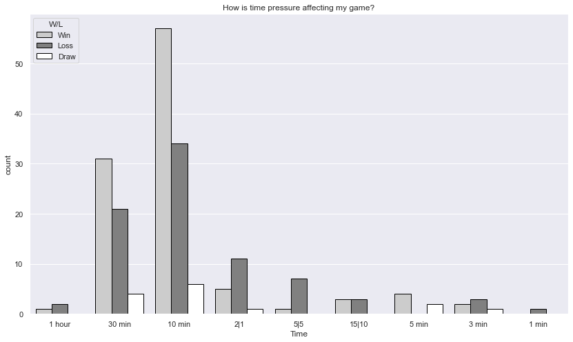
Overwhelmingly better at 30 and 10 minute games, quicker games fair much worse - a lesson to be learnt here, take your time and play long games.
Rating vs wins
fig = plt.figure(figsize=(14,8))
ax = fig.add_subplot(1,1,1)
ax.set_title("How does my rating affect wins?")

sns.histplot(games, x="My Rating", hue="Win", multiple="dodge", palette={0: "Black", 1: "Grey"})
plt.close(2)
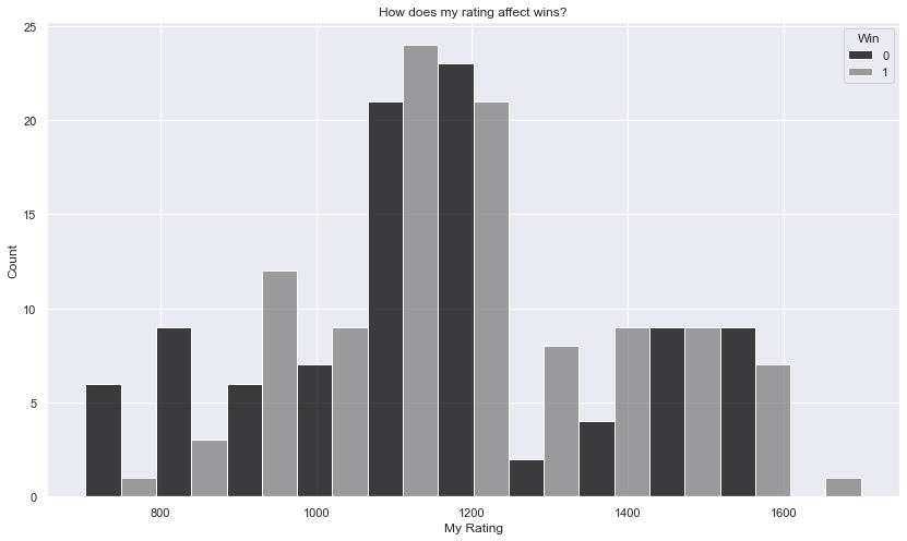
There is a pattern of high losses, then an increase in rating, higher wins then high losses again - this must be a development pattern in action. Importantly, must get more experience playing games at the higher level to match the 1000 - 1200 range. The 1400 - 1600 should be as high to be able to break into the 1600 - 1800 range.
Final words
I hope you enjoyed this tutorial. Now you have a way to monitor, track and analyse your Chess.com games archive to identify trends. Some of the actions this analysis has led me to are:
- Concentrating on improving on the endgame.
- Increasing my exposure to higher rated games.
- Strengthening play with the White pieces.
- Playing more consistently to ensure rating is accurate.
If there are any other analytical questions you'd like to ask of this dataset, let me know in the comments below and I'll update the article.
If you want to export the data to CSV you can use something like this on the games DataFrame:
path = os.path.join(os.path.dirname(os.getcwd()), 'my-chess-games-data.csv')
games.to_csv(path, index=False)