Exploring coding interview topics in Python

There are fundamental topics on algorithms and data structures that need to be understood for coding interviews. I am certainly no expert on coding interviews themselves, but I did embark on working through Elements of Programming Interviews in Python. I used this book in combination with it’s companion EPI-Judge and also LeetCode problems.
I did this to become better at programming in general and to brush up on algorithms and data structures. I’m not sure if you agree, but I feel (and have heard others say) that most of the time, the kinds of problems you find in programming interview questions are not the same as what actually occur on the job. Probably more of the job is focused on system design and architecture instead. Nevertheless, they have their merits and I admit they made me think more algorithmically and improved the efficiency of my code.
With all this in mind, in this article I’ve collated what I think are good examples mostly from LeetCode that help with learning and applying the concepts in the real world. They cover the major coding interview topics. It should be a good overview for those new to these topics, and a good reminder for those wishing to recap knowledge that might not have been used for a while. This is a long article you can use as a reference again and again - you can use the contents panel above to find your way back to the relevant section more easily.
Big-O Notation
Before diving into the topics and examples, it's important to understand Big-O Notation first. This allows us to assess the efficiency of an algorithm. For time complexity we ask how fast does the algorithm execute it's operations as the input size scales and becomes very large. For space complexity we ask how much memory will the algorithm consume as the input size scales and becomes very large. Space complexity consists of auxiliary space (space for extra variables and data structures we declare), input space (space for the given input) and stack space (for recursion). As the input size can vary, it is referred to as n. Below are the common notations you will see, with complexities ordered from smallest to largest, along with examples. These notations can be applied to both time and space complexity.

Constant time: O(1)
Where an algorithm does not depend on input size n, it runs in constant time. In this example, the loop will always run 100 times.
count = 0
for i in range(100):
  count += 1
print(count)
Other examples include accessing an array by index, adding or removing an element from an array, looking up a value in a dictionary (hashmap) and arithmetic operations.
Logarithmic time: O(log(n))
Where an algorithm's run time grows in proportion to the logarithm of the input size n. This means the algorithm isn't really affected by the input size and still runs rapidly on large inputs.
Using Binary Search to find an element in a sorted list is a good example. The algorithm uses a "divide and conquor" approach, it jumps to the middle of the list, divides the list into two and repeats until the element is found. So the algorithm is reducing the size of the input at each step therefore doesn't need to check every value.
n = 1000000
my_list = list(range(n)) # generates a list of numbers 0 through to "n"

def binary_search(array, target_value):
  list_length = len(array)
  left = 0
  right = list_length - 1
  while left <= right:
    middle = (left + right) // 2 # // performs integer division rather than floating-point division
    if target_value < array[middle]:
      right = middle - 1
    elif target_value > array[middle]:
      left = middle + 1
    else:
      return middle
  return "Search completed but value not found in array"

search_result = binary_search(my_list, 300000)
print(search_result)
This example searches a sorted array of integers 0 through to 1000000 (n). The algorithm sets a left and right index, then while the left index is lower than or equal to the right, checks whether the target value is less than the middle or greater than the middle, adjusting the left or right indexes accordingly to "split" the array. If the target value isn't less than or greater than the middle, we've found it and can just return middle 😄 This algorithm runs extremely fast even if the list input size n grows larger.
Linear time: O(n)
Where an algorithm depends on input size n, it runs in linear time.
n = 10000000
count = 0
for i in range(n):
  count += 1
print(count)
Linearithmic time: O(n log(n))
Where an algorithm uses a combination of linear and logarithmic time complexity. In the first place a linear search taking O(n) occurs followed by a reduction by half which means the next operation is O(log(n)) - we saw this "divide and conquer" approach used in Binary Search earlier. Therefore it's O(n*log(n)). Examples include Merge Sort, Quick Sort and Heap Sort. Let's implement Merge Sort to sort an array.
my_list = [54, 567, 26, 93, 17, 77, 31, 44, 55, 20, 44, 55, 14, 52]

def merge_sort(array: list):
  if len(array) > 1:
    # split the array into two
    print("Splitting", array)
    middle = len(array) // 2
    left = array[:middle]
    right = array[middle:]

    # recursive calls
    print("Recursing")
    merge_sort(left)
    merge_sort(right)

    # merge
    i = 0 # index to traverse the left array
    j = 0 # index to traverse the right array
    k = 0 # index for the main array

    # compare the left array and right array and
    # overwrite the main array with the lowest value
    print("Merging ", array)
    while i < len(left) and j < len(right):
      if left[i] < right[j]:
        array[k] = left[i]
        i += 1
      else:
        array[k] = right[j]
        j += 1
      k += 1

    # transfer all remaining values in the left array
    while i < len(left):
      array[k] = left[i]
      i += 1
      k += 1

    # transfer all remaining values in the right array
    while j < len(right):
      array[k] = right[j]
      j += 1
      k += 1

merge_sort(my_list)
print(my_list)  # [14, 17, 20, 26, 31, 44, 44, 52, 54, 55, 55, 77, 93, 567]
An initial array is divided into two roughly equal parts. If the array has an odd number of elements, one of those "halves" is by one element larger than the other. The subarrays are divided over and over again into halves until you end up with arrays that have only one element each. Then you combine the pairs of one-element arrays into two-element arrays, sorting them in the process. Then these sorted pairs are merged into four-element arrays, and so on until you end up with the initial array sorted. This CS50 video explains the process in more detail.
You can visualise Merge Sort through it's algorithm diagram. If you want some real fun you can check out what Merge Sort looks like in real time in this video.
Quadratic time: O(n²)
Where an algorithm has two nested loops / iterations, it runs in quadratic time.
n = 100
array_x = [42] * n  # list which is the length of "n" with all the same elements 42

def print_all_array_pairs(array_x):
  count = 0
  for i in range(len(array_x)):
    for j in range(len(array_x)):
      print(array_x[i], array_x[j])
      count += 1
  print(count)

print_all_array_pairs(array_x)
The final run count is 10000 for this example where n is 100. As 100^2 = 10000 so it's O(n²).
However a nested loop where the input sizes are different would be O(n*y).
x, y = 50, 100
array_x = [42] * x # list which is the length of "x" with all the same elements 42
array_y = [22] * y # list which is the length of "y" with all the same elements 22

def print_all_array_pairs(array_x, array_y):
  count = 0
  for i in range(len(array_x)):
    for j in range(len(array_y)):
      print(array_x[i], array_y[j])
      count += 1
  print(count)

print_all_array_pairs(array_x, array_y)
This is because the inner loop with a constant number of iterations is run y times for each iteration of the outer loop that is run x times. In this example the the outer loop runs for the length of array_x which is 50 and the inner loop runs for the length of array_y which is 100. So the final count is 5000 which is 50 x 100 therefore O(n*y).
Cubic time: O(n³)
Where an algorithm has three nested loops or iterations, it runs in cubic time. Here is an example I made to find the sum of all the numbers with three loops:
my_list = [44, 55, 63, 123, 54, 43, 34, 54] # "n" is the length of the list which is 8

def sum_all_numbers(array: list):
  sum_of_numbers = 0
  run_count = 0

  for i in my_list:
    sum_of_numbers += i
    for j in my_list:
      sum_of_numbers += j
      for k in my_list:
        sum_of_numbers += k
        run_count += 1
        print(i, j, k)

  return sum_of_numbers, run_count

result, run_count = sum_all_numbers(my_list)
print(f"Sum with three nested iterations: " + str(result)) # Summing this list across three nested loops is 34310
print("Run count: " + str(run_count)) # Run count where "n" is 8 is 8^3 so 512
The print statements helps to visualise what's happening as i j and k iterate over the list. As the list in this example has a length of 8 then n = 8. We're iterating over the list with three loops so the time complexity is O(n³), therefore the total executions stored in run_count is 8^3 or 8x8x8 which is 512.
Exponential time: O(2^n)
Where an algorithm's run time doubles with each addition to the input. Iterating through subsets comes to mind here. A good example is the use of a recursive algorithm to calculate Fibonacci numbers. The Fibonacci sequence is where each number is the sum of the two preceding numbers starting from 0 and 1. So 0, 1, 1, 2, 3, 5, 8, 13, 21, 34, 55, 89, 144, ... So if we set n = 9, the 9th number in the sequence starting from 1 is 34, and this runs very fast. But what if we want the 40th number in the sequence?
import time

def find_nth_number_in_fibonacci_sequence(n):
    if n <= 1:
        return n
    return find_nth_number_in_fibonacci_sequence(n - 2) + \
           find_nth_number_in_fibonacci_sequence(n - 1)

n = 40
start = time.time()
print(find_nth_number_in_fibonacci_sequence(n)) # 40th number in the fibonacci sequence is 102334155
end = time.time()
print(f"Time taken: {end - start} seconds") # This took 59.58 seconds for me
You can see the greater the number in the sequence you're looking for, the more recursive calls are required. You can better visualise what's happening in a recursion diagram. In the Dynamic Programming / Memoization section later in the article, we'll look at how to dramatically improve this run-time.
Factorial time: O(n!)
Where an algorithm's run time increases factorially with the increase in input size. A quick refresher on what a factorial is:
the product of all positive integers less than or equal to a given positive integer and denoted by that integer and an exclamation point. Thus, factorial seven is written 7!, meaning 1 × 2 × 3 × 4 × 5 × 6 × 7. - Britannica
So to find the factorial of a number n using a recursive approach has n factorial or O(n!) time complexity. We can see this algorithm will perform exponentially more operations as the input size increases (calculating the factorial of all positive integers before n)
def find_factorial(n):
  if n == 1:
    return n
  else:
    return n * find_factorial(n - 1)
Now that we've covered Big-O Notation and the common time complexities, we can dive into the topics 😆
Arrays
Definition: An array (list in Python) is a data structure that holds a group of elements, usually of the same data type (but not always) - like this [1, 2, 3, 4, 5]
Example Problem: Chunk an array into a given size n.
Example Input: [1, 2, 3, 4, 5, 6, 7], size=3
Example Output: [[1, 2, 3], [4, 5, 6], [7]]
import math

def chunk(collection: list, size: int) -> list:
  result = []
  count = 0

  for i in range(math.ceil(len(collection) / size)):
    start = i * size
    end = start + size
    result.append(collection[start:end])
    count += 1

  print(count)
  return result

if __name__ == "__main__":
  print(chunk([1, 2, 3, 4, 5, 6, 7], size=2))
  print(chunk([1, 2, 3, 4, 5, 6, 7], size=3))
  print(chunk([1, 2, 3, 4, 5, 6, 7], size=4))
Explanation: On each iteration a new start and end index is defined, and the array is sliced then added to the new result array. The run time of this algorithm is O(n) as the loop runs the length of collection n/size, each loop runs a slice operation of size using start and end. So the time complexity is n/size * size which is n.
Practical use: A practical use of an algorithm like this I have seen is creating a navigation tile layout on a webpage. Of course there are libraries that fulfil this need too, but why not implement it yourself to cut down your list of dependencies 😄 This is the first example I could find to illustrate.

This is how we might make use of the algorithm to achieve it.
chunks = chunk(["Wellbeing", "Healthy weight", "Exercise", "Sleep", "Eat well", "Alcohol support"], size=3)
  for chunk in chunks:
    for index, item in enumerate(chunk):
      print(item, end="\n") if index == 2 else print(item, end=", ")
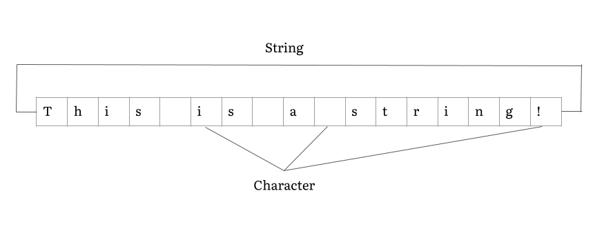
Strings
Definition: Strings can be thought of as an array, but made up of characters
Example Problem: Reverse String (Leetcode 344)
Example Input: hello
Example Output: olleh
class Solution:
    def reverseString(self, s: List[str]) -> None:
        """
        Do not return anything, modify s in-place instead.
        """
        left = 0
        right = len(s) - 1

        while left < right:
            temp = s[left]
            s[left] = s[right]
            s[right] = temp

            left += 1
            right -= 1
Explanation: Using a two pointer approach we start from the left and right, swapping each character with the help of a temporary variable, eventually meeting in the middle.
Linked Lists
Definition: A linked list is a linear collection of data elements similar to an array, but the order is not given by their physical placement in memory. A linked list can be singly or doubly linked.

Example Problem: Merge Two Sorted Lists (Leetcode 21)
Example Input: l1 = [1,2,4], l2 = [1,3,4]
Example Output: [1,1,2,3,4,4]
# Definition for singly-linked list.
# class ListNode:
#     def __init__(self, val=0, next=None):
#         self.val = val
#         self.next = next
class Solution:
    def mergeTwoLists(self, l1: ListNode, l2: ListNode) -> ListNode:
        dummy = ListNode(0)
        head = dummy

        while l1 and l2:
            if l1.val < l2.val:
                dummy.next = l1
                l1 = l1.next
            else:
                dummy.next = l2
                l2 = l2.next

            dummy = dummy.next

        if l1 != None:
            dummy.next = l1
        else:
            dummy.next = l2


        return head.next
Explanation: We are asked to return a sorted list by merging two sorted linked lists. We create a dummy head node, then while both l1 and l2 are not None, we assign the lower of the two as the dummy.next node and move them along. This builds up our new linked list in sorted order. When we break out of the while loop, we check which one has the leftover node (still not None) and assign it as the last node in the chain. Finally, returning head.next to avoid the first dummy node we created 😄
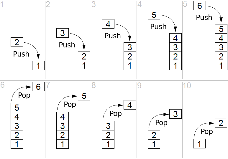
Stacks
Definition: A stack holds an ordered, linear sequence of items. In contrast to a queue, a stack is a last in, first out (LIFO) data structure. It is also used to implement depth first search.
Example Problem: Min Stack (Leetcode 155)
Example Input: ["MinStack","push","push","push","getMin","pop","top","getMin"]
Example Output: [[],[-2],[0],[-3],[],[],[],[]]
class MinStack:
    def __init__(self):
        """
        initialize your data structure here.
        """
        self.stack = []
        self.min_stack = []

    def push(self, val: int) -> None:
        self.stack.append(val)
        val = min(val, self.min_stack[-1]) if len(self.min_stack) > 0 else val
        self.min_stack.append(val)

    def pop(self) -> None:
        self.stack.pop()
        self.min_stack.pop()

    def top(self) -> int:
        return self.stack[-1]

    def getMin(self) -> int:
        return self.min_stack[-1]


# Your MinStack object will be instantiated and called as such:
# obj = MinStack()
# obj.push(val)
# obj.pop()
# param_3 = obj.top()
# param_4 = obj.getMin()
Explanation: To keep track of and lower the expense of retrieving the minimum element, we implement a two stack approach. The main stack holds the entries and the min stack holds the current minimum value, which updates during push with either the new value or the popped minimum value, whichever is lower.
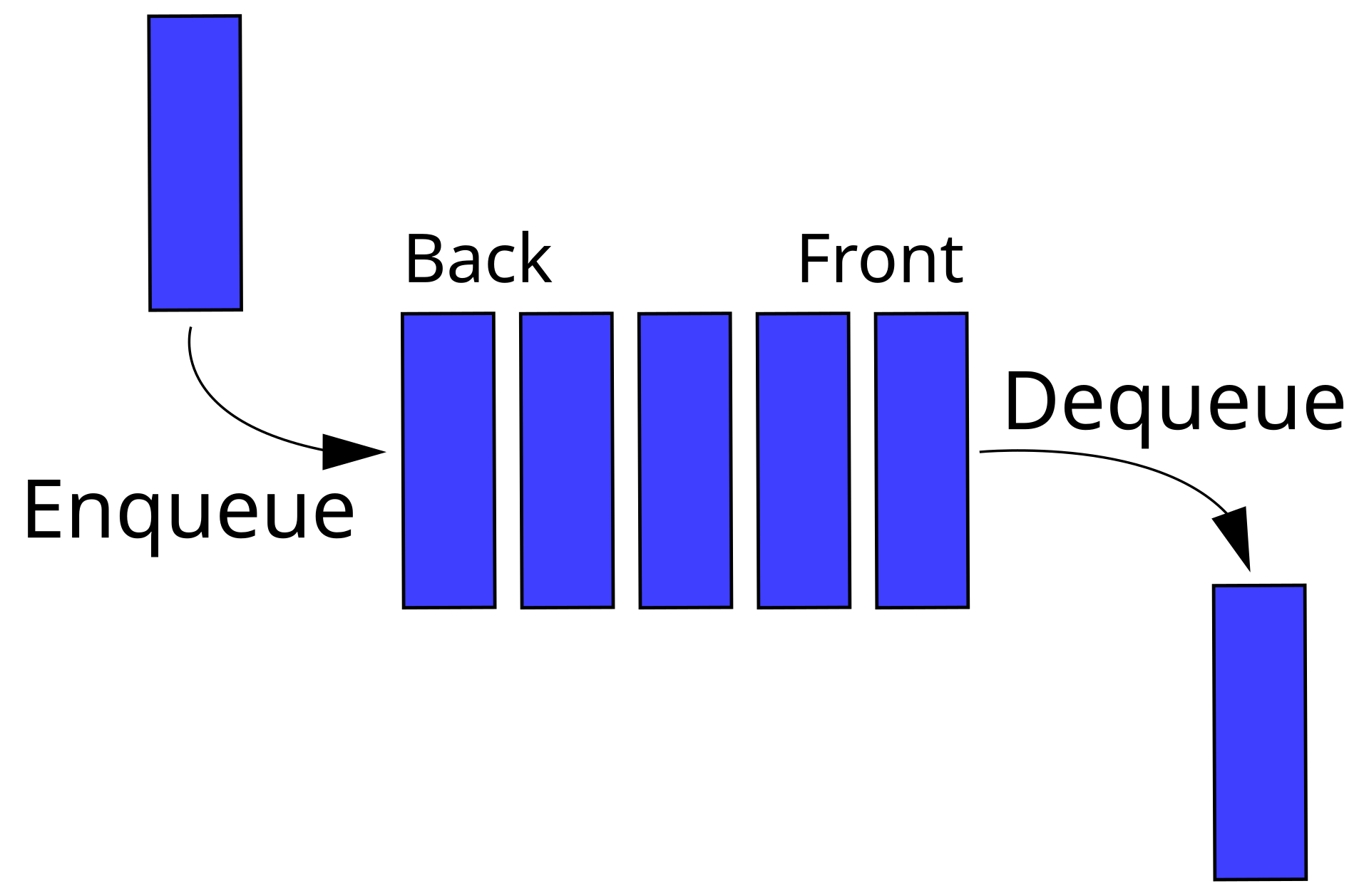
Queues
Definition: A queue holds an ordered, linear sequence of items. In contrast to a stack, a queue is a first in, first out (FIFO) data structure. It is used to implement breadth first search.
Example Problem: Binary Tree Level Order Traversal (Leetcode 102)
Example Input: root = [3,9,20,null,null,15,7]
Example Output: [[3],[9,20],[15,7]]
# Definition for a binary tree node.
# class TreeNode:
#     def __init__(self, val=0, left=None, right=None):
#         self.val = val
#         self.left = left
#         self.right = right
import collections

class Solution:
    def levelOrder(self, root: TreeNode) -> List[List[int]]:
        result: List[List[int]] = []

        if root == None:
            return result

        # Initialise queue and add first node
        queue: Deque[int] = collections.deque()
        queue.append(root)

        # Loop over queue
        while not len(queue) == 0:
            current_level = []
            for i in range(len(queue)):
                current_node: TreeNode = queue.popleft()
                current_level.append(current_node.val)
                if (current_node.left):
                    queue.append(current_node.left)

                if (current_node.right):
                    queue.append(current_node.right)

            result.append(current_level)

        return result
Explanation: We create a queue frontier to implement breadth first search and append the root node. Then at each iteration we clear the queue appending everything to the current_level before expanding the node's left and right children. To understand the difference between using a queue or stack as a frontier watch this video from CS50 AI.
Heaps
Definition: A heap is a data structure like a tree with the interesting property that any node has a lower value than any of its children (min-heap) or any node has a higher value than any of its children (max-heap).
Example Problem: Last Stone Weight (Leetcode 1046)
Example Input: [2,7,4,1,8,1]
Example Output: 1
import heapq

class Solution:
    """
    See https://docs.python.org/3/library/heapq.html for heapq docs
    """
    def lastStoneWeight(self, stones: List[int]) -> int:
        heap = [-abs(x) for x in stones] # negative value as heapq is min heap by default
        heapq.heapify(heap)

        while len(heap) > 1:
            stone_one = abs(heapq.heappop(heap))
            stone_two = abs(heapq.heappop(heap))

            if stone_one != stone_two:
                heapq.heappush(heap, -abs(stone_one - stone_two))

        heap_is_empty = len(heap) == 0

        return 0 if heap_is_empty else abs(heapq.heappop(heap))
Explanation: Our brief is if x == y, both stones are destroyed, and if x != y, the stone of weight x is destroyed, and the stone of weight y has new weight y - x. At the end of the game, there is at most one stone left. We create a heap list with the negative value of the stones (because heapq is a min-heap by default we need to turn that into a max-heap). Then heapq.heapify(heap) transform the list in-place. We then pop the two heaviest stones from the max-heap and if not equal add back their difference, not forgetting to make the value negative. If they are the same we do nothing (both stones were destroyed). We then just need to check if any stones are left with heap_is_empty and if it is return the last stone's weight 😄
HashMaps or Dictionaries
Definition: A hashmap or hashtable (dictionary in Python) is a data structure that implements an associative array abstract data type - a structure that can map keys to values, like this { "name": "John", "age": "44" }
Example Problem: Valid Anagram (Leetcode 242)
Example Input: s = "anagram", t = "nagaram"
Example Output: true
There are a few valid solutions for this - we'll start with the fundamental example of using a hashmap, then simplify.
class Solution:
    def isAnagram(self, s: str, t: str) -> bool:
        if len(s) != len(t):
            return False

        counter = {}

        for letter in s:
            if letter in counter.keys():
                counter[letter] += 1
            else:
                counter[letter] = 1

        for letter in t:
            if letter not in counter.keys():
                return False

            if counter[letter] < 1:
                return False

            counter[letter] -= 1


        return True
class Solution:
    def isAnagram(self, s: str, t: str) -> bool:
        return Counter(s) == Counter(t)
class Solution:
    def isAnagram(self, s: str, t: str) -> bool:
        return sorted(s) == sorted(t)
Explanation: Wikipedia tells us 'An anagram is a word or phrase formed by rearranging the letters of a different word or phrase, typically using all the original letters exactly once. For example, the word anagram itself can be rearranged into nagaram, also the word binary into brainy and the word adobe into abode'. We need to test if t is an anagram of s. In the first approach, implement a counter ourselves, counting each character in s and storing the count in a dictionary. We then go over each letter in t decrementing from the count. If the letter isn't in the dictionary, or the count drops below zero we know it's not a valid anagram. Approach two simplifies this to use Python's built in Counter to compare both strings. As the order of the words don't matter, we could also sort the strings then compare them as in the third approach.
The commonly used data structures for hashmaps in Python are set, dict, collections.defaultdict and collections.Counter.
Searching
Definition: A search algorithm is used to find specific data within a data structure.
Example Problem: Binary Search (Leetcode 704)
Example Input: nums = [-1,0,3,5,9,12], target = 9
Example Output: 4
class Solution:
    def search(self, nums: List[int], target: int) -> int:
        left, right = 0, len(nums) - 1

        while left <= right:
            middle = (left + right) // 2

            if nums[middle] == target:
                return middle

            if target > nums[middle]:
                left = middle + 1
            else:
                right = middle - 1


        return -1
Explanation: For our example input, 9 exists in nums and its index is 4. To satisfy a O(log n) runtime complexity, we implement binary search. We keep finding the middle, if it is the target we return it's index, else when the target is greater than the middle we replace the left index with the middle or the right index when less than the middle. This effectively cuts the array in half every time until we find the target or leave the while loop.
Sorting
Definition: A sorting algorithm re-organises a data structure into a specific order, such as alphabetical, highest-to-lowest value or shortest-to-longest distance.
Example Problem: Intersection of Two Sorted Arrays II (Leetcode)
Example Input: nums1 = [4,9,5], nums2 = [9,4,9,8,4]
Example Output: [4,9] or [9,4]
class Solution:
    def intersect(self, nums1: List[int], nums2: List[int]) -> List[int]:
        if len(nums1) > len(nums2):
            return self.intersect(nums2, nums1)

        map: dict = {}

        for number in nums1:
            if number in map.keys():
                map[number] += 1
            else:
                map[number] = 1

        intersection: List = []

        for number in nums2:
            count: int = map[number] if number in map.keys() else 0

            if count > 0:
                intersection.append(number)
                map[number] -= 1


        return intersection
or by using Counter we saw in the hashmaps section with it's elements() method ...
class Solution:
    def intersect(self, nums1: List[int], nums2: List[int]) -> List[int]:
        if len(nums1) > len(nums2):
            return self.intersect(nums2, nums1)

        nums1_count = Counter(nums1)
        nums2_count = Counter(nums2)

        return (nums1_count & nums2_count).elements()
Explanation: The intersection is everything that nums1 and nums2 have in common. We must ensure each element in the result must appear as many times as it shows in both arrays. In the first approach we create our own counter map to count the occurance of each number in nums1. Then for each number in nums2 we check if it's in the dictionary and if it is append it to the intersection list then decrement the count by one. We can then return the intersection as the answer. Approach two simplifies this by using Counter.
Graphs
Definition: A graph represents a non-linear relationship between it's nodes which are connected by edges.

Example Problem: Clone Graph (Leetcode 133)
Example Input: adjList = [[2,4],[1,3],[2,4],[1,3]]
Example Output: [[2,4],[1,3],[2,4],[1,3]]
"""
# Definition for a Node.
class Node:
    def __init__(self, val = 0, neighbors = None):
        self.val = val
        self.neighbors = neighbors if neighbors is not None else []
"""

class Solution:
    def cloneGraph(self, node: 'Node') -> 'Node':
        if not node:
            return None

        map: dict = {}

        def dfs(node, map):
            if node in map:
                return map[node]

            print(f"Copying node {node.val}")
            copy = Node(val=node.val)
            map[node] = copy

            for neighbor in node.neighbors:
                print(f"Appending neighbour node {neighbor.val} to node {copy.val}")
                copy.neighbors.append(dfs(neighbor, map))

            return copy


        return dfs(node, map)
Explanation: We are asked to effectively manually implement copy.deepcopy(node) to copy the contents of a graph given it's entry node. We initialise a dictionary map to store and return the copied nodes we've already seen. If we've not already seen the node, we create a copy and store it, then for each of it's neighbours append them as the copy's neighbours using depth first search and recursion with dfs. This clones every node and in turn copies the neighbors of each node.
Bitwise manipulation
Definition: Bitwise manipulation performs a logical operation on each individual bit of a binary number.
Preparation: To solve these problems you must first know the bitwise operators and converting binary numbers to denery and denery numbers to binary. It is also useful to understand signed and unsigned numbers and least significant bit.
Here is a concise bitwise operators reference table I stapled together from various sources.
| Operator | Syntax | Meaning | Description | Example |
|---|---|---|---|---|
| & | a & b | Bitwise AND | Returns 1 if both the bits are 1 else 0 | 1010 & 0100 = 0000 |
| | | a | b | Bitwise OR | Returns 1 if either of the bit is 1 else 0 | 1010 | 0100 = 1110 |
| ^ | a ^ b | Bitwise XOR (exclusive OR) | Returns 1 if one of the bits is 1 and the other is 0 else returns false. | 1010 ^ 0100 = 1110 |
| ~ | ~a | Bitwise NOT | Returns one’s complement of the number | ~1010 = -(1010 + 1) = -(1011) = -11 (decimal) |
| << | a << n | Bitwise left shift | Shifts the bits of the number to the left and fills 0 on voids left as a result. | 0000 0101 << 2 = 0001 0100 |
| >> | a >> n | Bitwise right shift | Shifts the bits of the number to the right and fills 0 on voids left as a result. | 0000 0101 >> 2 = 0000 0001 |
Example Problem: Counting Bits (Leetcode 338)
Example Input: 9
Example Output: 2
A good example to illustrate bitwise manipulation is counting bits set to 1 in a positive integer. The Leetcode example is an array of positive integers - so the same solution but for each item in the array.
def count_bits(x: int) -> int:
    num_bits = 0
    while x:
        num_bits += x & 1   # checks if the rightmost bit is 1 (0001 & 0001 = 1)
        x >>= 1             # shifts the number right one bit, shifting out the least significant bit

    return num_bits

count_bits(9) # Returns 2
Explanation: If we take the number 9, which in binary is 1001, then we can see there are two bits set to 1.
- We start with 1001 and add
x & 1(1001 & 0001 = 0001) tonum_bitswhich now has a count of 1 (1 added) - Then shift the bits right making 0100 and repeat adding
x & 1(0100 & 0001 = 0000) tonum_bitswhich now has a count of 1 (nothing added). - Then shift the bits right making 0010 and repeat adding
x & 1(0010 & 0001 = 0000) tonum_bitswhich now has a count of 1 (nothing added). - Then shift the bits right making 0001 and repeat adding
x & 1(0001 & 0001 = 0001) tonum_bitswhich now has a count of 2 (1 added). xis now 0 so the while loop exits and the returned count ofnum_bitsis 2! 😄
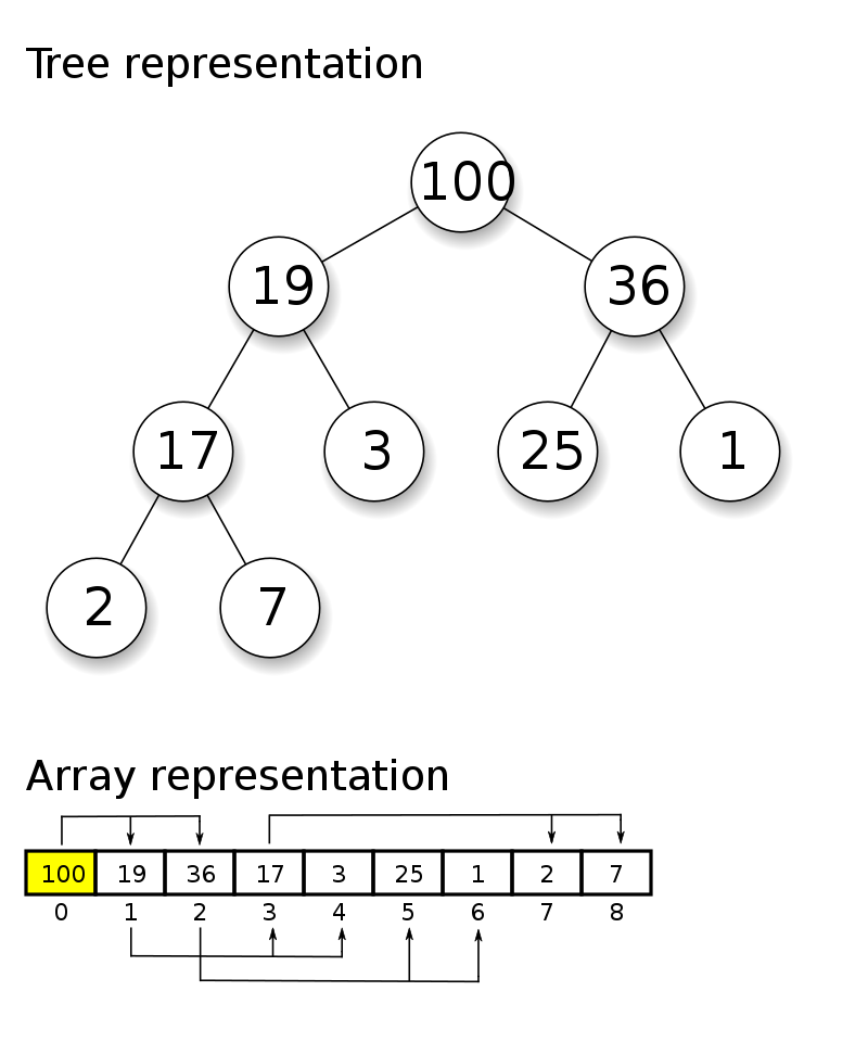
Binary Trees
Definition: A binary tree is a tree data structure in which each node has at most two children, which are referred to as the left child and the right child.

Example Problem: Balanced Binary Tree (Leetcode 110)
Example Input: root = [3,9,20,null,null,15,7]
Example Output: true
Here I've presented the code along with the explanation in an image, to visualise what's going on.
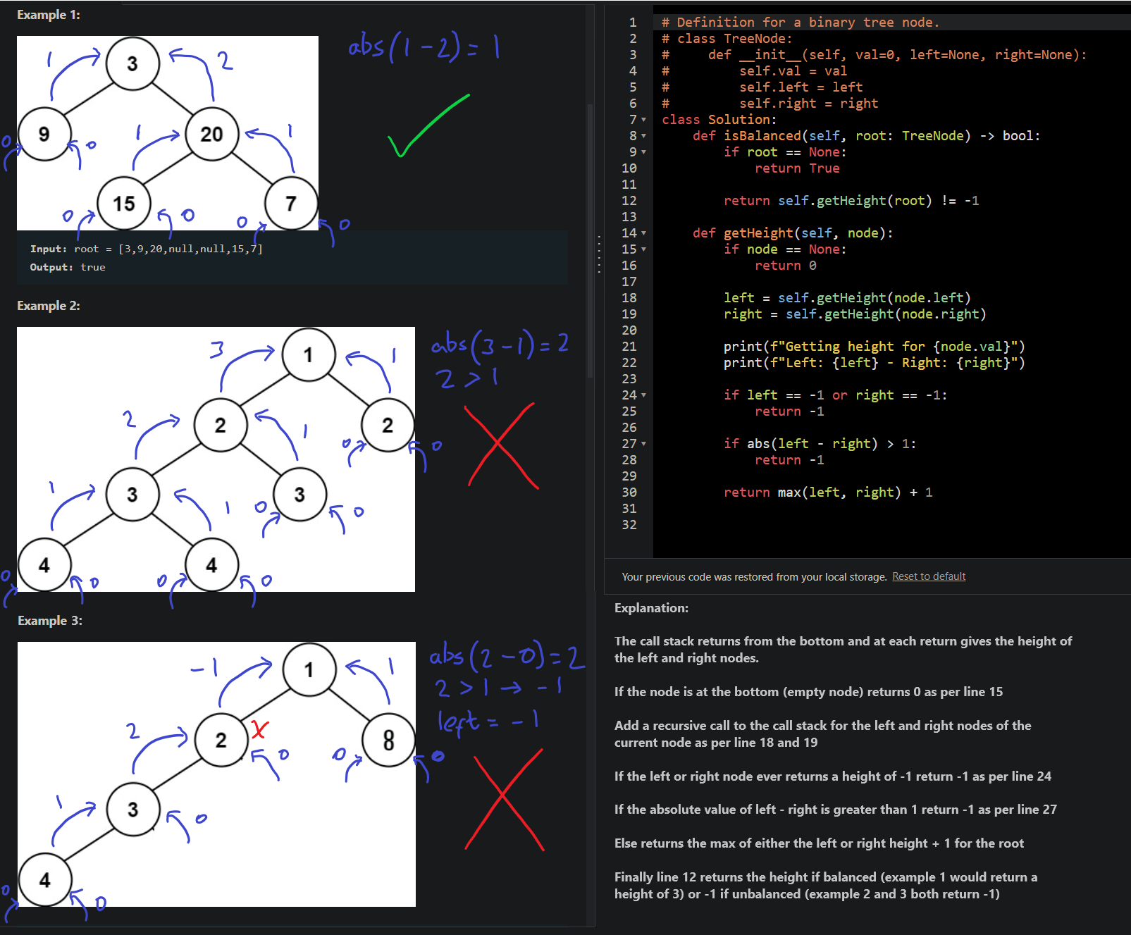
Explanation: A binary tree is balanced when the left and right subtrees of every node differ in height by no more than 1. We use recursion (covered later) to carry out postorder traversal to ensure every subtree is balanced all the way back to the top. If that's a bit confusing this video goes into more detail.
Binary Search Trees
Definition: Binary search tree (BST), also called an ordered or sorted binary tree, is a rooted binary tree data structure whose internal nodes each store a key greater than all the keys in the node’s left subtree and less than those in its right subtree.

Example Problem: Validate Binary Search Tree (Leetcode 98)
Example Input: [2,1,3]
Example Output: true
# Definition for a binary tree node.
# class TreeNode:
#     def __init__(self, val=0, left=None, right=None):
#         self.val = val
#         self.left = left
#         self.right = right
class Solution:
    def isValidBST(self, root: Optional[TreeNode]) -> bool:

        def validate(node: TreeNode, lower_bound: float, upper_bound: float):
            if not node:
                return True

            node_in_bounds = node.val < upper_bound and node.val > lower_bound
            if not node_in_bounds:
                return False

            return (
                validate(node.left, lower_bound, node.val) and
                validate(node.right, node.val, upper_bound)
            )

        return validate(root, float("-inf"), float("inf"))
Explanation: We need to determine if a binary tree is a valid binary search tree (BST) given it's root node. Any node must be greater than all the keys in it's left subtree and less than those in it's right subtree. We can use depth first search and recursion to validate each node is within the lower_bound and upper_bound. This ensures that if a left or right subtree falls out of bounds it is not a valid BST.
Recursion
Definition: Recursion is a process in which a function calls itself as a subroutine, thereby dividing a problem into subproblems of the same type.
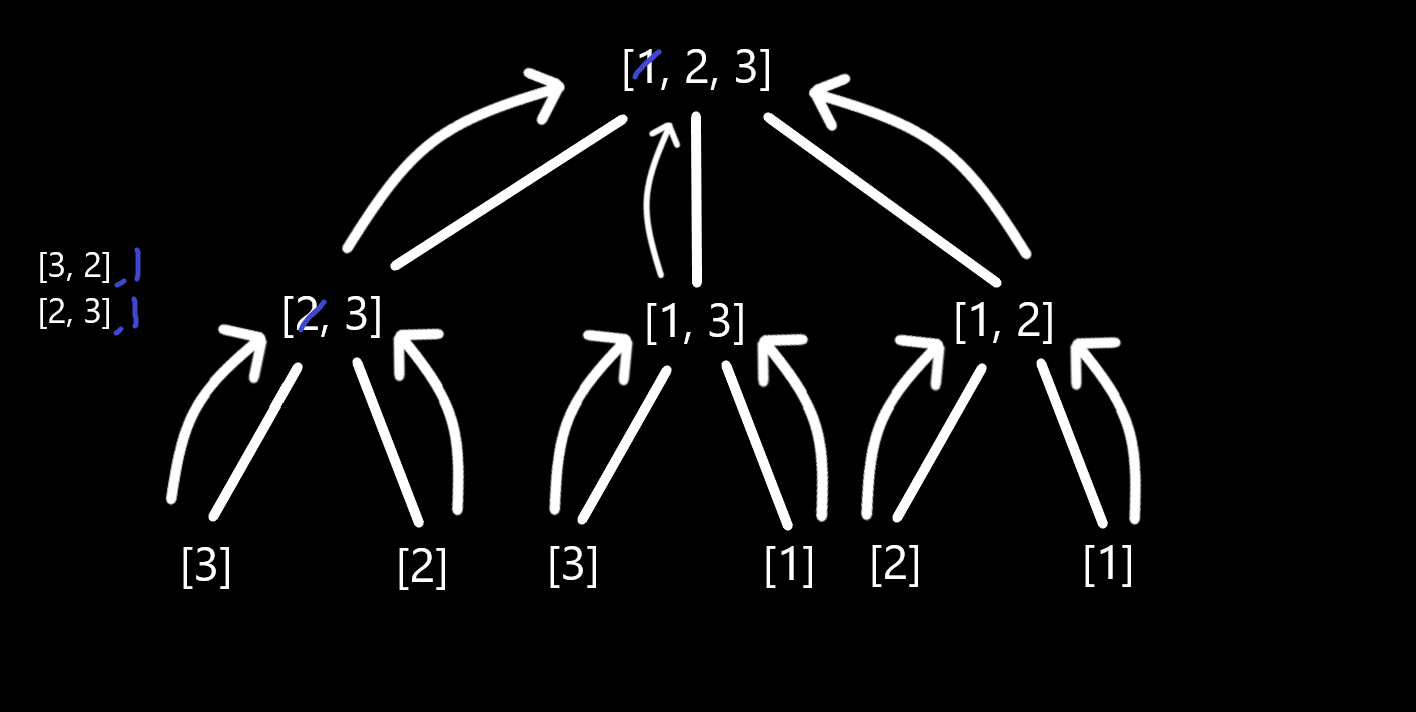
Example Problem: Permutations (Leetcode 46)
Example Input: nums = [1,2,3]
Example Output: [[1,2,3],[1,3,2],[2,1,3],[2,3,1],[3,1,2],[3,2,1]]
class Solution:
    def permute(self, nums: List[int]) -> List[List[int]]:
        result: List[List[int]] = []

        if len(nums) == 0:
            return [nums[:]]

        for i in range(len(nums)):
            number = nums.pop(0)
            permutations = self.permute(nums)

            for permutation in permutations:
                permutation.append(number)

            result.extend(permutations)
            nums.append(number)

        return result
Explanation: We are asked to return all the possible permutations of nums in any order. So for each integer in nums [1,2,3] we pop the first element leaving [2,3] and then call permute again (recursively) to get each sub-permutation. This would leave us with [3,2] and [2,3] so now we append the popped number back the the permutation, giving [3,2,1] and [2,3,1] and add both of these to the result using extend(). Finally, we append the popped number back to nums. This will repeat for each element giving all possible permutations. The magic of recursion right? Here is a diagram to visualise the process that will be carried out for each. We always pop the first element, then get permutations, add the element back, extend the result, append the element back.
Dynamic Programming or Memoization
Definition: Dynamic programming is a technique for solving problems of recursive nature, iteratively and is applicable when the computations of the subproblems overlap. Memoization is a term describing an optimization technique where you cache previously computed results, and return the cached result when the same computation is needed again.
Example Problem: Fibonacci Number (Leetcode 509)
Example Inputs: n = 40
Example Output: 102334155
Earlier when discussing Big-O Notation I used an example find_nth_number_in_fibonacci_sequence to demonstrate exponential time O(2^n). In the example I tried to find the 40th number in the fibonacci sequence using recursion and this took a huge 59.58 seconds. The greater the number in the sequence we were looking for, the more the runtime grew exponentially. How can we improve this? What about using memoization to cache the results of each recursive call so no unnecessary repeat calls are ever made.
import time

def find_nth_number_in_fibonacci_sequence(n, cached_results: dict):
    if n in cached_results.keys():
      return cached_results[n] # return result if already in cache

    if n <= 1:
        result = n
    else:
      result = find_nth_number_in_fibonacci_sequence(n - 2, cached_results) + \
               find_nth_number_in_fibonacci_sequence(n - 1, cached_results) # ensure cache is passed to all recursive calls

    cached_results[n] = result # cache the result
    return result

start = time.time()
n = 40
print(find_nth_number_in_fibonacci_sequence(n, dict())) # 40th number in the fibonacci sequence is 102334155
end = time.time()
print(f"Time taken: {end - start} seconds") # This took 0.0009975433349609375 seconds for me
Explanation: Modifying the code we used earlier to include a cache in the form of a dictionary, to find the 40th number in the sequence it now takes 0.0009975433349609375 seconds for me!! By caching and reusing earlier results the speed has improved dramatically. Using a hashmap (dictionary) to lookup cached results has a constant time complexity of O(1).
Final thoughts
So now you should have a good idea of the data structures and algorithms included in a coding interview. This might not prepare you for one (only constant focused practice can do that) but it will make you aware of what you don’t know. I have been doing problems on LeetCode and EPI and trying to really understanding the solution before moving on. A key part of this strategy has been tracking performance and repeating failed problems. Here is my Trello board when I first started.
The approach was to add problems for each topic we've covered to the Problems list, then each day move 3-5 problems across to the Doing list. Once attempted, I rated performance out of 5 (5 being perfect with no help needed, 1 being didn't finish it without help and further study) and move it to the Repeat list (worst at the top). Then on subsequent days take another 3-5 problems from the Problems list, and one from the top of the Repeat list. Rinse and repeat. The idea came from this Engineering with Utsav video (I really like this channel).This has allowed me to focus on breath of knowledge, whilst revisiting and repeating weaker areas.
More so than passing any test, I hope this article gives you the inspiration to become an (even) better programmer and to think more algorithmically. As always if you have any thoughts let me know in the comments section below. Alternatively, you can complete the site's new feedback form - you might have noticed the new 👍 feedback button on the navbar, so you can say how you think the site is doing and what you would like to see more of in the future 😄
Resources
- Python Standard Library Reference
- Elements of Programming Interviews | Book
- EPI-Judge
- LeetCode
- Grokking Algorithms
- Computer Science Distilled
- Big-O Examples in Python
- Time Complexity Examples in Python
- Memoization and Dynamic Programming Explained
- Bitwise Operators
- Data Structures & Algorithms in Python | Excellent but expensive, might be able to find an e-book version cheaper
- 10 Important Data Structures & Algorithms for Interviews
- Understanding Merge Sort in Python